Understanding Convolutional Neural Network
 |
- It uses weight sharing concept due to which the number of parameters that needs training is substantially reduced, resulting in improved generalization.
- Due to lesser parameters, It usually do not suffer overfitting.
- Here the classification stage is incorporated with feature extraction stage.
- The performance is remarkable.
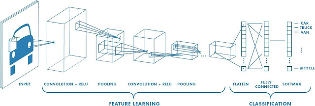
CNN consists of one or more convolutional layers which is followed my single or more connected layers. It is designed in such a way that it can take advantage of 2D structure of an image to the fullest. CNN are used widely in domains like image classification, Object Detection, face detection, vehicle recognition, facial expression recognition and many more. Recently CNN is also discovered to have excellent capacity in sequent data analysis such as natural language processing.
There are mainly two operations in CNN namely convolution and pooling.
The convolution operation is responsible for feature extraction from the dataset, through which their corresponding spatial information can be preserved.
The pooling also called subsampling is responsible for reduction of dimensionality of feature maps from convolution operation.
General Model of Convolution Neural Network
Traditionally, an ANN(Artificial Neural Network) has one input and a output layer along with numbers of hidden layers. CNN is based on contextual information and it consists of four different components as:
- Convolution Layer
- Pooling Layer
- Activation Function
- Fully Connected Layer
1. Convolution Layer
If a image is to be classified It is sent as input and the output is predicted class computed using extracted feature image. Each neuron is connected to other neuron in previous layer or the next layer, this correlation is termed as receptive field using which forms a weight vector from where image feature is extracted. The weight vector aka filter/kernel slides over the input vector to generate the feature map. This sliding operation is called as convolution. The formula for convolution is as follow:
 |
2. Pooling Layer
After the feature map is extracted it is sent to pooling layer. It remarkably reduces number of trainable parameters and introduces translation invariance. To Perform pooling a window is selected and the input elements lying in that window are passed through the pooling function as below:
This pooling function generates another output vector. There are numbers of pooling techniques like average pooling and max pooling among them max-pooling is most popular technique since it significantly reduces the map-size.
3. Fully Connected Layer
The output from above layer is sent to this layer. Here, dot product of weight vector and input vector is calculated. Gradient descent aka batch mode learning aka offline algorithm reduces the cost function by estimating the cost over an entire training dataset and update the parameter after only one epoch. If the dataset is too large the time required to train increases substantially. In that case stochastic gradient descent are used.
4. Activation Function
Different kind of activation functions are used in CNN depending on the case. Among such functions sigmoid function is the most popular one. In case of non-linearity Rectified Linear Unit(ReLU) has proven itself better than other.
Architectures of Convolutional Neural Network
Various architecture have been introduced and implemented in CNN. Here is the Brief explanation to some popular ones:
1. LeNet Architecture
LeCun et al. introduced the LeNet architecture in their 1998 paper, Gradient-Based Learning Applied to Document Recognition. This architecture consists of 8 layers among which five are convolutional layers and remaining are fully connected layers. This architecture is pretty straightforward. and It can run on both CPU and GPU.
 |
| LeNet Architecture |
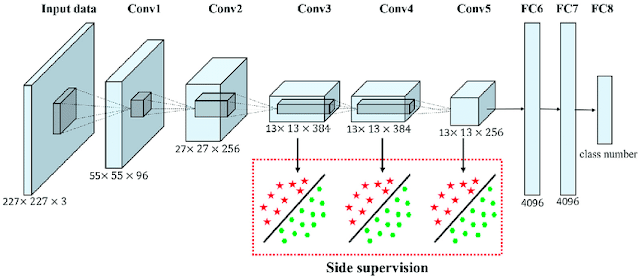
2. AlexNet Architecture
In 2012, three scientists from University of Toronto introduced Alexnet in their paper Imagenet Classification with Deep Convolutional Neural Networks which reduced the top 5 error of other architecture from 26% to 15.3%. This architecture is very similar to LeNet but with deeper filters per layer and with stacked convolutional layers. It has 11*11, 5*5, 3*3, convolutions, max pooling, dropout, data augmentation, ReLu activation Function. It connected Relu after each convolutional and fully connected layer.
3. GoogleNet Architecture
GoogleNet architecture is proposed in 2014 by a team of researcher from Google in their paper Going Deeper with Convolutions. This paper was winner of ILSVRC 2014 image classification challenge. This architecture is very different from other architectures. It achieved a top five error rates of 6.67 %. It uses various kind of models as follow:
ZFNet was introduced in 2013 paper Visualizing and Understanding Convolution Networks. This paper is the winner of 2013 ILSVRC.
5.VGGNet
VGGNet was introduced in 2014 in the paper Very Deep Convolutional Networks For Large-Scale Image Recognition. It was the runner-up of ILSVRC 2014.
6.ResNet
ResNet was first introduced in the paper Deep Residual Learning for Image Recognition at ILSVRC 2015.
Learning Algorithm
Learning algorithms aka optimizing algorithms improves the network by minimizing loss function aka objective function biased on various learnable parameters such as weight, bias etc. Basically learning algorithm can be categorized into first order and second order optimization algorithms.
First Order Optimizing Algorithm include the calculation of gradient represented by Jacobian matrix. this technique is widely used in Gradient Descent.
Second Order Optimizing Algorithm consists of second order derivatives represented by Hessian matrix. Adam optimization make wide use of this technique.
Refrences:


Post a Comment